main menu | module menu | << previous section | next section >>

TCAD to SPICE
6. Garand MC

6.1 Overview
6.2 Command Files and Initial Guess
6.3 Solution Approaches
6.4 Monte Carlo Simulation Parameters
6.5 Monte Carlo Output
6.6 Garand Material Model
6.7 Quantum Corrections
6.8 Example: 2D MOSFET

Objectives

To become familiar with the capabilities of Garand MC.
To introduce the structure of input files that Garand MC uses.

6.1 Overview

Garand Monte Carlo (MC) is a three-dimensional, self-consistent, ensemble quantum corrected device simulator that uses the Monte Carlo approach to solve the Boltzmann transport equation and is capable of both electron and hole transport in a range of materials.

This approach is non-local and non-equilibrium, accurate for small channel lengths and for high fields. Additionally, the impact of stress and material composition is captured directly through the band structure, allowing it to properly predict transport in contemporary and future semiconductor devices. In contrast, a standard drift-diffusion approach is a local, equilibrium approach that is reliant on mobility models to describe carrier transport, limiting its ability to be predictive, especially in scaled transistors.

The solution from Monte Carlo simulation is provided through the collection of statistical data taken from particle distributions representing the electron and/or hole carrier distributions within the simulation domain. The particle distribution evolves during the simulation by the repeated application of periods of deterministic free flight and instantaneous stochastic scattering events. Carriers move through the real-space simulation domain during free flight and given a local field, accelerate, while scattering from a list of mechanisms affects the carrier momentum. Self-consistency is provided by solving the Poisson equation at regular intervals to obtain the electrostatic potential consistent with the simulated particle distribution. Ensemble average properties such as velocity, energy, or current can be extracted from the gathered data.

Garand MC can be used to simulate transport in a range of domains from simple bulk material through to full device simulation in a range of semiconductor materials and compounds (group IV, III-V, III-N) to assess low and high field transport properties, extract full I-V curves to predict on-current, or provide target data for calibration of drift-diffusion or SPICE models. Internal distributions of carriers, scattering or average energy can be extracted, and device ballisticity can be assessed to provide better understanding of the transport underlying the predicted device performance.

6.2 Command Files and Initial Guess

The initial guess and domain for a Garand MC simulation comes from a prior drift-diffusion simulation. The initial guess is used to define the boundary conditions in line with the applied bias for a device simulation, along with the Density Gradient quantum corrections which remain fixed for the duration of the Garand MC simulation.

To use the drift-diffusion simulator that is installed with Garand MC, select the "PRE" radio button in the Garand MC Tool Properties window:

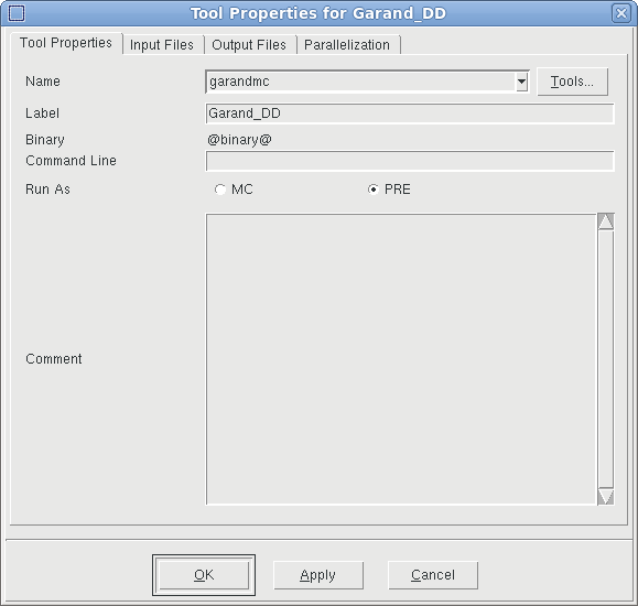
Tool Properties for initial drift-diffusion simulation

Figure 1. Enabling the drift-diffusion simulator installed with Garand MC.

To run a Monte Carlo transport simulation, select the "MC" radio button:

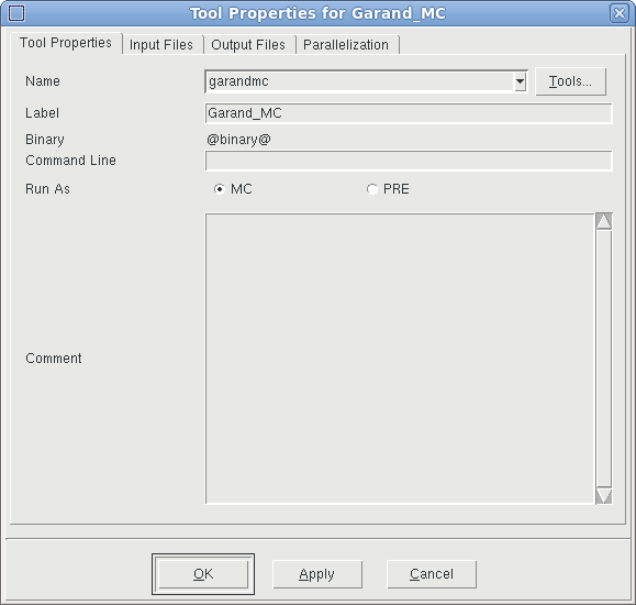
Tool Properties for Garand MC simulation

Figure 2. Enabling a Monte Carlo transport simulation with Garand MC.

Alternatively, Sentaurus Device can be used to supply the initial guess, which is transferred via a TDR file. The following fields must be written out by Sentaurus Device when it is supplying an initial guess to Garand MC:

DonorConcentration AcceptorConcentration eDensity hDensity ElectrostaticPotential ElectronAffinity EffectiveBandGap eEffectiveStateDensity hEffectiveStateDensity

There are additional, optional fields which are required when specific models are enabled in Garand MC.

Where quantum corrections are used, the following fields are required:

eQuantumPotential hQuantumPotential

Where trapped charge is included in the simulations, each of the following fields may be imported:

fixedCharge eInterfaceTrappedCharge hInterfaceTrappedCharge

To import stress or mole fraction fields, the following fields should be written to TDR:

Stress xMoleFraction

There are two input files connected to each Garand MC tool instance:

Commands: The input file specific to a given stage
Base Garand Input File: A shared input file for all Garand MC simulations, used to ensure consistency of common models and parameters

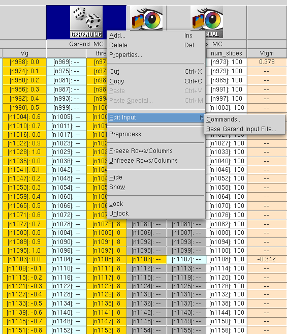
Figure 3. Accessing the stage specific command file and the base input file shared between all Garand MC stages.(Click image for full-size view.)

It is recommended that the base input file contains only commands that are general across all Garand MC stages (both PRE and MC), and commands specific to a stage are contained in the Commands file. Testing the @toolname@ variable to apply specific settings should be avoided for clarity.

Minimum requirements for device simulation:

Base Garand Input File

Set bias conditions.
Import contacts and set workfunction.
Set type (n or p)
For running in SWB, set flags to ensure output is written to correct folder.

An example of a minimal base input file is given below:

#----------------------- LOCAL PREPROCESSOR DEFINITIONS ------------------------
#if "@Type@" == "nMOS"
#define _n_or_p_     n

#elif "@Type@" == "pMOS"
#define _n_or_p_     p                                                          
#else
puts "Type is incorrect... @Type@"
#endif

#------------------------------- BIAS CONDITIONS -------------------------------
BIAS        gate        = @Vg@                                                  
BIAS        drain       = @Vd@                                                 
BIAS        substrate   = 0.0                                                   

#------------------------------ CONTACT DEFINITION -----------------------------
CONTACT     metal_gate import = 'gate'                                          
CONTACT     source     import = 'source'                                        
CONTACT     drain      import = 'drain'                                        
CONTACT     substrate  import = 'substrate'                                    

CONTACT     work_function     = @WF@                                            

#------------------------------- SIMULATION MODEL ------------------------------
SIMULATION  n_or_p            = _n_or_p_                                        

#------------------------------ OUTPUT PARAMETERS ------------------------------
OUTPUT      hierarchical      = off                                             
OUTPUT      experiment        = n@node@

Command File (initial guess)

Import base input file.
Import structure from a Sentaurus Process simulation or Sentaurus Structure Editor.
Specify the source of the mesh - either import from the structure file or define locally.
Set flag to ensure TDR is written with a solution that can be imported as initial guess for Garand MC.

An example of a minimal command file for the initial guess, simulated with Garand MC, is given below:

#--------------------------- GARAND BASE INPUT FILE ----------------------------
IMPORT      pp@node@_gmc.garinp                                                 

#------------------------------ SIMULATION DOMAIN ------------------------------
STRUCTURE   IMPORT  filename = @[relpath n@node|MOS@_msh.tdr]@                 

#------------------------------- MESH DEFINITION -------------------------------
MESH        IMPORT                                                            

# ------------------------------ SIMULATION OUTPUT -----------------------------
OUTPUT      mc_transfer = on

Command File (MC simulation)

Import base input file.
Import initial guess from prior drift-diffusion simulation.
Set at least one carrier type to be simulated (electron or hole) and enable super particles.

An example of a minimal command file for Monte Carlo simulation is given below:

#--------------------------- GARAND BASE INPUT FILE ----------------------------
IMPORT      pp@node@_gmc.garinp                                                 

#------------------------------ SIMULATION DOMAIN ------------------------------
STRUCTURE   IMPORT   filename=@[relpath n@node|Garand_DD@-DD-Output_1.tdr]@     

# ---------------------- MONTE CARLO SIMULATION PARAMETERS ---------------------

SIMULATION  superparticles          = on                                        

#if "@Type@" == "nMOS"
SIMULATION  electrons               = on                                        

#elif "@Type@" == "pMOS"
SIMULATION  holes                   = on                                        
#endif

While this minimal set of commands, in most cases, allows simulations to run and complete, further commands are generally required to ensure quality of results and to reduce turnaround time. A more comprehensive set of command files is described in the example below.

6.3 Solution Approaches

Where device current is the main result, there are three approaches that can be used with Garand MC:

Self-consistent ensemble MC (EMC) propagates an ensemble of carriers in time, while continuously solving the electrostatic potential. The transient behaviour of the ensemble is recovered as it reaches steady state.

For EMC, convergence is strongest above threshold, but as the current is a statistical measure convergence can be poor where the current is small, such as in the subthreshold. This requires significant computational overhead to resolve an accurate measure of the current often resulting in longer turn around times.

To enable an EMC simulation, specify the following:
```
SIMULATION ensemble = on
```
Backward MC (BMC) propagates a limited set of carriers from the virtual source back to the device contacts, where the probability of the corresponding forward trajectory is determined, allowing the device current to be estimated.

Where the current is low, BMC converges in significantly less time than EMC, making it particularly suitable for simulation in the subthreshold regime. The accuracy of the result is dependent on the fixed potential which is typically supplied by the initial guess. The potential from the prior drift-diffusion solution is more likely to be accurate in the subthreshold.

To specify a BMC simulation:
```
SIMULATION backward_MC = on
```
Single-particle MC (SMC) propagates an ensemble of carriers in time but in a fixed potential. Carriers sample the steady state only and transient behaviour is not recovered.

To specify an SMC simulation:
```
SIMULATION single_particle = on
```

By default, both the EMC and BMC models are enabled, and Garand MC selects which model to apply based on a user definable current criterion applied to an initial estimate of the current using the initial guess. Where the current is below the threshold, BMC is used for the simulation (see Figure 4).

This approach allows the solution to be partitioned into two regimes:

Sub-threshold where BMC is used
Above threshold simulated using EMC

This partitioning allows the appropriate solution approach to be used where it is strongest, improving convergence and reducing the overall turnaround time.

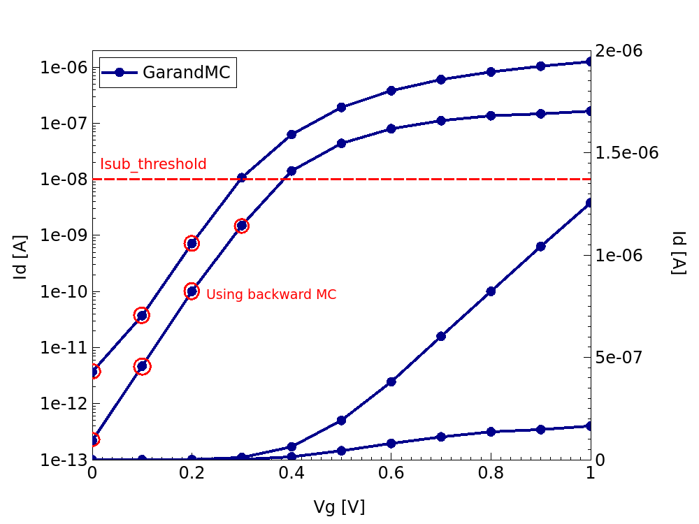
Figure 4. Id-Vg characteristics from Garand MC simulation highlighting the threshold below which BMC is used and the bias points simulated with this approach.(Click image for full-size view.)

6.4 Monte Carlo Simulation Parameters

The initial guess from an earlier drift-diffusion simulation defines both electron and hole carrier densities. Either or both species can be resolved as particles and simulated with Monte Carlo, using the following commands:

SIMULATION electrons = on
SIMULATION holes = on

As a minimum requirement, at least one carrier type must be specified in the command file.

The number of particles used to resolve the continuous carrier distribution imported from drift-diffusion can either be defined so that either:

Each particle represents a single charge.
Each particle represents multiple or fractional charges.

The former is the default, but to switch to the case where each carrier represents a nonunity charge, set the following flag:

SIMULATION superparticles = on

In this case, the number of carriers used can be set separately for each carrier species using the following commands:

SIMULATION num_elec = 200000
SIMULATION num_hole = 200000

Increasing the number of particles allows for better sampling of the current, less noise in the result, and improved convergence, but at the cost of a greater run time, in particular for simulations of hole transport.

The number of carriers required for a simulation depends on the size of the domain (3D or quasi 2D) and the doping density in the source and drain. Aiming for at least 1 particle per mesh element in the source and drain regions is generally a reasonable estimate.

The duration of a Monte Carlo simulation is determined by two aspects:

The specified maximum simulation time
Convergence criteria

The maximum simulation time is based on the maximum number of time steps (\(N_{steps}\)):

SIMULATION num_steps = 200000

and the propagation time step (\(Δt\)):

SIMULATION DT = 5.d-17

so that the maximum simulation time is \(t_{total} = Δt · N_{steps} = 10ps\) based on the values given above.

The propagation (or field-adjusting) time step defines the period over which particles propagate assuming a constant field. At the end of this step, electric fields are interpolated at the new position of the particle, updating the field for the next time step. Where the simulation is self-consistent, Poisson's equation is re-solved before the interpolation to update the electrostatic potential (and thus the field) based on the particle distribution at the end of the propagation step.

Care should be taken where adjusting both parameters that defines the maximum simulation time. For the propagation step:

Large values accumulate large errors making the simulation unreliable.
Small values are accurate but increase the turnaround time.

In general, good values for the time step are:

1e-15s for bulk material simulations where the field is constant or slowly varying.
5e-17s for device simulations, in particular which has quantum corrections.

The maximum number of time steps should then be set so the total simulation time is long enough to ensure the simulation reaches steady state and sufficient statistics can be gathered to minimize the uncertainty of the quantity of interest (for instance, current in device simulations). A total simulation time of 10ps is generally a reasonable maximum duration.

Convergent criteria can be defined to allow the simulation to exit early once the current converges within a requested tolerance. This can be set in the form of the relative error of the mean current, defined as a percentage:

SIMULATION tolerance = 1.0

or in the form of an absolute error in Amperes:

SIMULATION abstol = 1.d-10

In some cases, convergence can be slow, so it is possible to set a tolerance based on the change in the error (defined as a percentage):

SIMULATION improvement_tolerance = 0.5

In this case if the change in the error of the mean current is below 0.5% over successive steps, then the simulation stops.

Convergence criteria can only be defined based on the current, so is only applicable for device simulation. Where other measures are the required output (such as mobility), it is recommended to disable convergence:

SIMULATION converge = off

In addition to the total number of time steps, there are other intervals that can be defined via the command file:

Transient Time
- Time is needed for the Monte Carlo simulation to respond to the applied bias and reach steady state where the current can be accurately estimated.
- Garand MC automatically estimates where the transient period ends and the simulation enters steady state, allowing the estimation of the mean current and associated error to be estimated based only on the latter period.
- Other average ensemble properties, such as energy or velocity, may have transient times that differ from the current. There, it is possible for the user to define a transient period via the command file:
```
SIMULATION num_trans = 30000
```
- This user defined period is observed only if the user enforces it:
```
SIMULATION exclude_trans_stats = on
```
- Or if TDR output is requested:
```
OUTPUT MC_results = on
```
Statistical Sampling Interval
- Ensemble averages may be highly correlated, in particular where the time step is short such as in device simulation.
- Garand MC estimates and discards correlated data, but collecting statistics to be discarded introduces unnecessary computational overhead.
- Therefore, it is possible to increase the interval between steps where the statistics are gathered:
```
SIMULATION num_stats = 200
```
Intermittent Output Interval
- The frequency at which convergence is tested and output is written to screen and file is defined using the command:
```
SIMULATION num_inter = 10000
```
- Setting this value too low can be inefficient, while setting it too large can delay the end of the simulation by failing to detect convergence.
- Typically, setting this parameter to 1000 for bulk material simulations and 10000 for device simulations are reasonable estimates.

6.5 Monte Carlo Output

Garand MC creates two output directories for each simulation named data and rates.

At the end of the intermittent output interval, ensemble averages are written to screen and file. For simulations using BMC, only the current is returned.

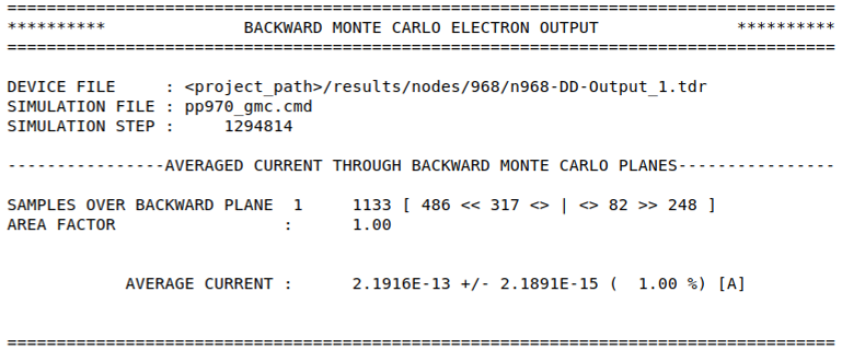
For simulations of electron transport, the output file is:

data/BACKWARD_MC_ELEC_OUTPUT

and for simulations of hole transport:

data/BACKWARD_MC_HOLE_OUTPUT

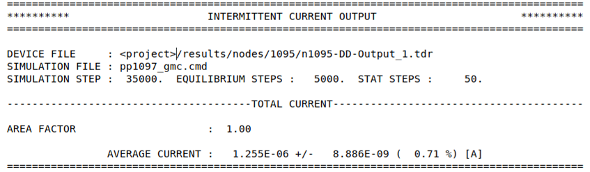
For EMC simulations, two files are written. The first reports only the current:

data/INTERMITTENT_CURRENT_OUTPUT

A second file reports a wider range of statistic from the EMC simulation based on the specified flags in the command file. For simulations including electron transport, this file is named:

data/INTERMITTENT_ELEC_OUTPUT

And for hole transport

data/INTERMITTENT_HOLE_OUTPUT

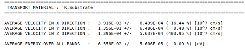
For instance, including the following flags instructs Garand MC to gather statistics on the average energy and velocity:

OUTPUT energy = on
OUTPUT velocity = on

Including the command:

OUTPUT time_evolution = on

Results in files with the average energy and velocity as a function of time to the data directory and the ensemble average for each region to be reported to the intermittent output file and to screen:

A log of scattering events for each valley is also reported as part of the intermittent output:

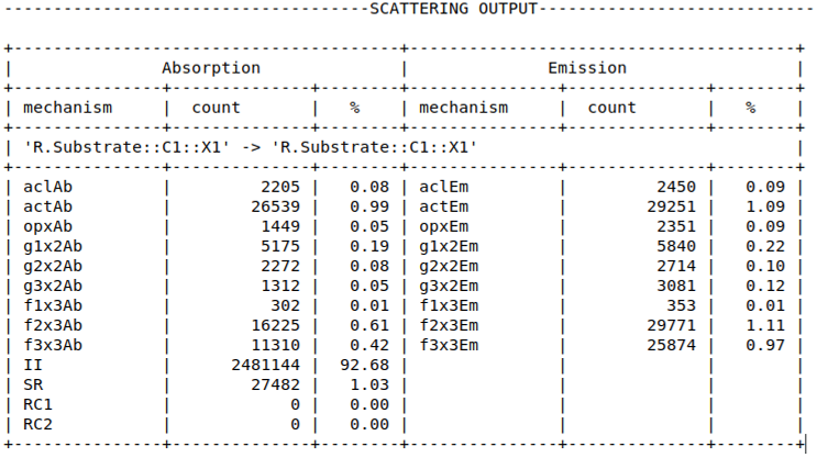
The scattering rate for each valley in each region can be written to the rates directory using the command:

OUTPUT scattering rates = on

To visualize the domain and initial guess, specify the following:

OUTPUT domain = on

This writes a TDR file named n@node@-MC_Input.tdr.

Similarly, to visualize the time-averaged fields in the steady state, use the following command:

OUTPUT MC_results = on

In this case, a TDR file named n@node@-MC-Output.tdr is written.

6.6 Garand Material Model

Materials can be thought of as a collection of objects in an object hierarchy and the command files provide the syntax for instantiation of new objects association of object parameter values. Parameters specific to a region within the domain can be modified directly by replacing the material name with the region name. For example, to modify the permittivity of Silicon:

MATERIAL Silicon.permittivity	2.0

This changes the permittivity of all Silicon regions. To subsequently modify the permittivity of a Silicon region named "Channel":

MATERIAL Channel.permittivity 4.1

All other Silicon regions retain the previously defined value and the Channel region uses 4.1.

For the bandstructure definition, each semiconductor material includes a conduction and valence band model that consists of a container that defines the nominal band edge and a list of bands. Each band then defines a dispersion model and a set of valley models. This is illustrated in Figure 5.

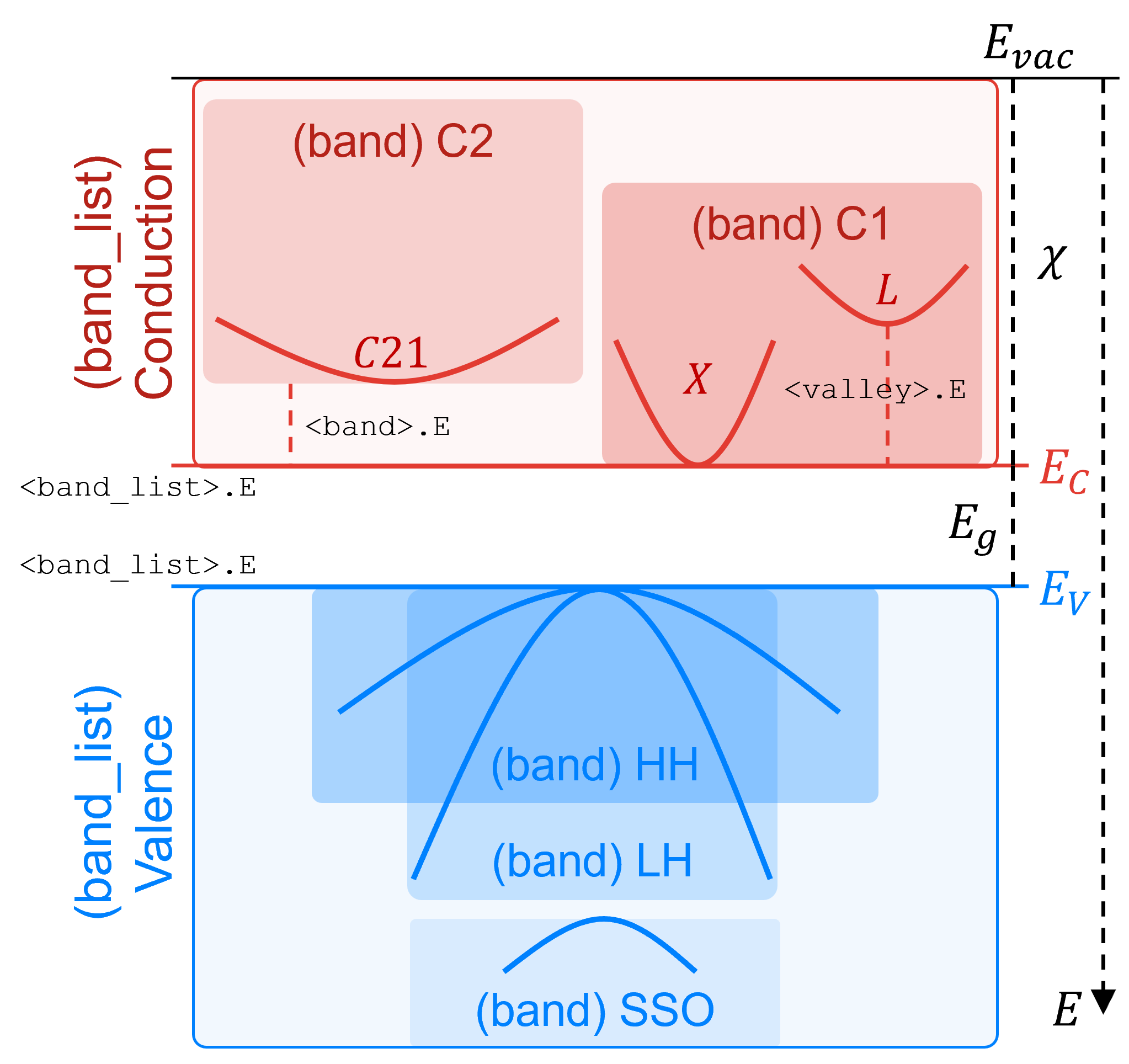
Figure 5. Bandstructure hierarchy in Garand, showing bands and valleys within the Conduction and Valence band containers. (Click image for full-size view.)

To modify a parameter within the conduction or valance band container model:

MATERIAL <material>.<band_list>.<parameter> <value>

where <band_list> can be conduction or valence.

The parameters for a given band can be modified as:

MATERIAL <material>.<band_list>.<band>.<parameter> <value>

And similarly, the parameters for a valley model can be modified as:

MATERIAL <material>.<band_list>.<band>.<valley>.<parameter> <value>

Member	Description
`<band_list>`	Minimum energy defined with respect to vacuum May contain an arbitrary number of bands
`<band>`	Minimum energy defined with respect to `<band_list>M` minimum May contain arbitrary number of valleys May be mapped to a full band calculation
`<valley>`	Minimum energy defined with respect to `<band>` minimum Mapped to local minimum in full band, if supplied

Scattering rates are tabulated for carriers in each valley as a function of carrier energy up to a user definable maximum:

MATERIAL <material>.<band_list>.<band>.<valley>.rates.E <value>

Parameters for each mechanism can be modified using similar syntax to that used to modify parameters related to the bandstructure:

MATERIAL <material>.<band_list>.<band>.<valley>.<mechanism>.<parameter> <value>

Scattering is defined from one valley to another with the mechanism active within its parent valley and scattering into a named final valley, with all valley names being unique across all bands (see Figure 6). For inelastic mechanisms, absorption and emission processes are defined.

Mechanisms must be defined for all equivalent valleys. Tcl scripting can be used to simplify the definition of scattering models or parameters:

foreach vi [list <initial valleys>] {
  foreach vf [list <final valleys>] {
    DEFINE   Silicon.Conduction.C1.${vi}.g1    OpPhon
    MATERIAL Silicon.Conduction.C1.${vi}.E     ${Eg1}
    MATERIAL Silicon.Conduction.C1.${vi}.final ${vf}
  }
}

The use of Tcl blocks like the one shown above is very useful in Garand MC command files to quickly define modifications or extensions to the existing material model. The order of the preprocessor execution means that the Tcl is executed first and so can be used to populate the command file with changes to the material model without having to explicitly introduce modifications by hand which can be cumbersome due to the completeness of the material model.

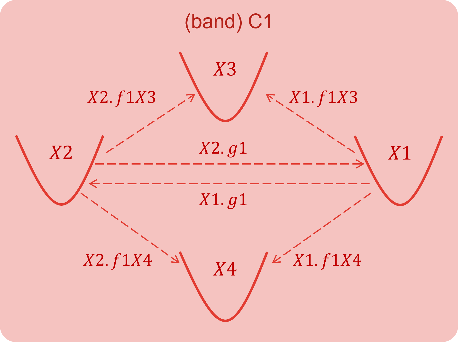
Figure 6. Illustration of inter valley scattering model in Garand. (Click image for full-size view.)

A list of scattering mechanisms available in Garand MC is given in the following table.

Scattering mechanisms	Models
Phonon scattering	Elastic/inelastic acoustic Polar and non-polar optical
Ionized impurity	Ridley's Third body Brooks-Herring
Surface roughness	Ando's model
Alloy
Remote Coulomb
Impact ionization	Keldysh model Kane Random-k model

A new scattering mechanism, for instance an optical phonon, includes the following in the command file. First define the type of mechanism (OpPhon) within the specific band (C1) and valley (G), and give it a name (opg):

DEFINE   GaAs.conduction.C1.G.opg       OpPhon

Then define parameters, in this case the phonon energy (E) and coupling constant (Cc):

MATERIAL GaAs.conduction.C1.G.opg.E     35.4e-3    
MATERIAL GaAs.conduction.C1.G.opg.Cc     2.100e10

And finally, specify the valley to scatter into - in this case this is an intravalley mechanism where the initial and final valleys are the same:

MATERIAL GaAs.conduction.C1.G.opg.final   G

For mechanisms associated with an interface, there are two steps. First, define the mechanism following a similar definition as for the optical phonon above, here for surface roughness scattering:

DEFINE   Silicon.conduction.C1.X1.SR         SR        
MATERIAL Silicon.conduction.C1.X1.SR.model   Ando     
MATERIAL Silicon.conduction.C1.X1.SR.final   X1

Then, define parameters for each semiconductor/insulator interface in the simulation domain, optionally specifying the carrier type (carrier) and surface orientation (orient) they relate to:

DEFINE Silicon.Oxide.rough_001 rough_interface
INTERFACE Silicon.Oxide.rough_001.carrier electrons
INTERFACE Silicon.Oxide.rough_001.orient 0 0 1 
INTERFACE Silicon.Oxide.rough_001.RMS 1.2 
INTERFACE Silicon.Oxide.rough_001.L 2.0

Interface parameters can be associated with a carrier type (electron or hole) and for a surface orientation, but they are the same for all valleys in the bandstructure model.

It is possible to filter the set of defined scattering mechanisms in all valleys associated with the conduction or valence band using the scattering parameter. This allows for mechanisms to be conveniently disabled or enabled on a per-material or per-region basis. Multiple filters can be defined in succession in a command file which are applied in the order they are defined.

For instance, to remove surface roughness scattering from all Silicon regions for electrons in the conduction band:

MATERIAL Silicon.conduction.scattering -sr

Then, re-introduce this mechanism to the region named "Channel" only:

MATERIAL Channel.conduction.scattering +sr

A list of available semiconductor materials for simulation with Garand MC is given in the following table.

Semiconductor materials
Silicon	SiliconGermanium
Germanium	InGaAs
GaAs	InAlAs
InAs	InP
AlAs	GaAsSb
GaN	GaSb
AlInN	AlGaN
InGaN	AlN
InN

Default material definitions are installed at:

$STROOT/tcad/current/linux64/lib/GARAND/materials/

The material definitions used in Garand MC are written to a file for inspection:

@node|Garand_MC@/data/Material_parameters.dat

As part of the material model, the bandstructure approximation used for electron and hole transport is set:

For all materials, default is the effective mass approximation (EMA) for electron transport.
For Silicon, SiliconGermanium, and Germanium, the 6kp model is used for hole transport.
- For all other materials, hole scattering models and parameters are not defined in the default model.

6.7 Quantum Corrections

A quantum correction is applied to the self-consistent electrostatic potential obtained from the solution of Poisson's equation resulting in a time-varying effective quantum potential that defines the driving field used in particle propagation.

The quantum correction is obtained from the initial drift-diffusion simulation and remains fixed through the Garand MC simulation.

Where Garand MC is used to provide the initial guess in PRE mode, the quantum correction is obtained through the solution of the density gradient equation, which is solved when the following is included in the command file:

MODEL density_gradient = on

Inclusion of this command in the Garand MC input file enables the application of the quantum correction in the transport simulation.

6.8 Example: 2D MOSFET

In the following section the demo project on Garand MC simulation for a 2D Si MOSFET is described.

This project can be investigated from within Sentaurus Workbench in the directory Applications_Library/GettingStarted/tcadtospice/garandmc/MOS_2D.

The flow, illustrated in Figure 7, consists of the following steps:

Sentaurus Structure Editor: creates NMOS and PMOS structures.
Garand MC "PRE": performs initial DD solution for a single bias point.
Garand MC: Runs Monte Carlo simulation at same bias point as previous step.
Gather data to plot I-V curves.
Process .tdr files to extract carrier-weighted profiles along the channel.

Figure 7. Tool flow for 2D MOSFET example in Sentaurus Workbench, showing the Sentaurus Structure Editor stage, 2 Garand MC steps and 2 Sentaurus Visual stages. (Click image for full-size view.)

The structure is a 2D planar Si MOSFET. The Garand MC stages introduces uniform 2GPa compressive stress to the PMOS simulation which the NMOS is unstressed. The doping profile and device structure for each is shown in Figure 8.

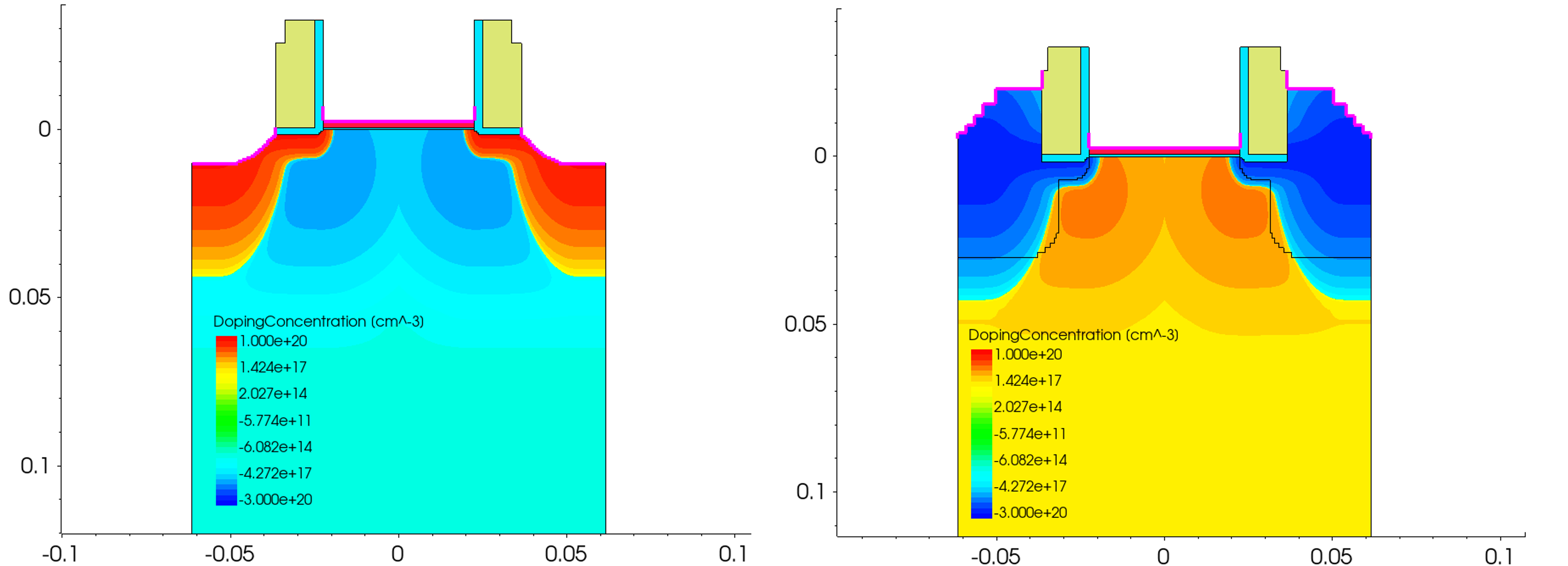
Figure 8. Device structure and doping profile for the 2D MOSFET example - NMOS (left) and PMOS (right). (Click image for full-size view.)

6.8.1 Base Garand Input File

The base Garand input file is used by all Garand MC stages (both the PRE and MC modes). It is used to define parameters that are common to all stages - these are generally adjustments to material or bandstructure parameters, but parameters specific to a given stage should be placed in the relevant command file.

The layout of the file is as follows:

At the top of the file, parameters relating to density gradient and the device type are set using the #define command.
The contacts are then mapped to fields in the imported TDR file and the work function set.
Bias conditions are then set to values defined as Sentaurus Workbench parameters.
Simulation parameters are defined - the temperature, simulation type, and density gradient quantum corrections are enabled.
Output parameters are set - hierarchical output is disabled for Garand MC so that output is written directly to the Sentaurus Workbench node folder. An experiment name is defined that is used to prepend output files.
A scaling factor for the current is set. In this case, it is set to 1.0.
A stress tensor is defined, with the stress in the channel direction set to a value defined as a Sentaurus Workbench parameter.
Finally, the higher valleys in the conduction band are removed because they are not occupied in this simulation. Removing them simplifies the output of the simulation and has no impact on the result.

#===============================================================================
# SIMULATION PARAMETERS COMMON TO BOTH DD AND MC SIMULATION
#===============================================================================
#----------------------- LOCAL PREPROCESSOR DEFINITIONS ------------------------
#define _chan_dir_   dgy       /* Define axis along channel direction [x/y/z] */

#if "@Type@" == "nMOS"
#define _n_or_p_     n         /* Set NMOS simulation */

#elif "@Type@" == "pMOS"
#define _n_or_p_     p         /* Set PMOS simulation */
#else
puts "Type is incorrect... @Type@"
#endif

#------------------------------ CONTACT DEFINITION -----------------------------
CONTACT     metal_gate import = 'gate'      # Define gate      contact
CONTACT     source     import = 'source'    # Define source    contact
CONTACT     drain      import = 'drain'     # Define drain     contact
CONTACT     substrate  import = 'substrate' # Define substrate contact

CONTACT     work_function     = @WF@        # Define the gate workfunction

#------------------------------- BIAS CONDITIONS -------------------------------
BIAS        gate              = @Vg@        # Gate      bias [V]
BIAS        drain             = @Vd@        # Drain     bias [V]
BIAS        substrate         = 0.0         # Substrate bias [V]

#------------------------------- SIMULATION MODEL ------------------------------
SIMULATION  T                 = 300         # Lattice temperature [K]
SIMULATION  n_or_p            = _n_or_p_    # n-type or p-type simulation

MODEL       density_gradient  = on          # Density gradient solution

#------------------------------ OUTPUT PARAMETERS ------------------------------
OUTPUT      hierarchical      = off         # Write to hierarchical directories?
OUTPUT      experiment        = n@node@     # Prefix for file names

#------------------------------ SIMULATION DOMAIN ------------------------------
STRUCTURE   AreaFactor        = 1.0         # Scaling factor for output current

#------------------------------ STRESS DEFINITION ------------------------------
STRAIN      Silicon.device_stress_tensor 0 @Syy@ 0 0 0 0 transfer_average=off

#---------------------------- MATERIAL REDEFINITION ----------------------------

# Remove higher conduction valleys as generally unoccupied
!(
  set matList [list Silicon]
  set valList [list L1 L2 L3 L4 L5 L6 L7 L8 G]

  foreach mat $matList {
    foreach val $valList {
      puts "MATERIAL    ${mat}.conduction.${val}     REMOVE "
    }
  }
)!

6.8.2 Command File for the Initial Guess

The command file for supplying the initial guess using the drift-diffusion solution of Garand MC is described in this section.

To alternatively use Sentaurus Device to provide the initial guess, the following steps are required:

Use a tensor product mesh.
Ensure that a TDR is written with the fields described above.
Produce a TDR per bias point to be simulated with Garand MC.

As with the base input file, parameters are set at the top of the file that are used in subsequent parameter or model definitions.

#===============================================================================
# GARAND DRIFT-DIFFUSION SIMULATION OF 2D DEVICE STRUCTURE.
# THE RESULT IS USED AS THE INITIAL STATE FOR ENSEMBLE MONTE CARLO SIMULATION
#===============================================================================
#setdep @node|MOS@

#----------------------- LOCAL PREPROCESSOR DEFINITIONS ------------------------
#if "@Type@" == "nMOS"
#define _band_       conduction   /* Set band for parameter modification */

#elif "@Type@" == "pMOS"
#define _band_       valence      /* Set band for parameter modification */
#else
puts "Type is incorrect... @Type@"
#endif

#--------------------------- GARAND BASE INPUT FILE ----------------------------
IMPORT      pp@node@_gmc.garinp   # Common setup for DD and MC simulation

#------------------------------ SIMULATION DOMAIN ------------------------------
STRUCTURE IMPORT filename = @[relpath n@node|MOS@_msh.tdr]@ # Relative path to 
                                                            # simulation domain 
                                                            # Tdr file

#------------------------------- MESH DEFINITION -------------------------------
MESH        IMPORT                # Import mesh from simulation domain Tdr file

#------------------------------- SIMULATION MODEL ------------------------------
SIMULATION  gummel_acc  = 1e-5    # Gummel loop accuracy
SIMULATION  epspois     = 1e-7    # Gummel Poisson solution accuracy
SIMULATION  epscurr     = 1e-9    # Gummel Current continuity accuracy
SIMULATION  epsdg       = 1e-7    # Gummel Density gradient accuracy
SIMULATION  iter_max    = 300     # Maximum number of Gummel iterations allowed

# ------------------------------ SIMULATION OUTPUT -----------------------------
OUTPUT      mc_transfer = on      # Write Tdr file with required fields for MC

#-------------------------------- MOBILITY MODEL -------------------------------
!(
  set matList [list Silicon]

  foreach mat $matList {
    puts "MATERIAL    ${mat}._band_.mobility.bulk    Masetti"
    puts "MATERIAL    ${mat}._band_.mobility.eprp    Yamaguchi"
    puts "MATERIAL    ${mat}._band_.mobility.elat    Caughey"
    puts "MATERIAL    ${mat}._band_.mobility.strain  SSE"
  }
)!

6.8.3 Command File for MC Simulation

As with the base input file, the MC command file sets parameters at the top that are used in subsequent parameter or model definitions, this time including defining directions related to the simulation domain that are used when setting the crystallographic orientation.

#===============================================================================
# GARAND MONTE CARLO SIMULATION OF 2D DEVICE STRUCTURE.
# - BACKWARD MC SOLUTION IS AUTOMATICALLY USED IN THE SUB-THRESHOLD REGION
# - EMSEMBLE MC SOLUTION USED OTHERWISE
#===============================================================================
#setdep @node|Garand_DD@

#----------------------- LOCAL PREPROCESSOR DEFINITIONS ------------------------
#define _chan_dir_   y      /* Define axis along channel    direction [x/y/z] */
#define _horiz_dir_  z      /* Define axis along horizontal direction [x/y/z] */
#define _vert_dir_   x      /* Define axis along vertical   direction [x/y/z] */

#if "@Type@" == "nMOS"
#define _band_       conduction        /* Set band for parameter modification */

#elif "@Type@" == "pMOS"
#define _band_       valence           /* Set band for parameter modification */
#else
puts "Type is incorrect... @Type@"
#endif

#--------------------------- GARAND BASE INPUT FILE ----------------------------
IMPORT      pp@node@_gmc.garinp          # Common setup for DD and MC simulation

#------------------------------ SIMULATION DOMAIN ------------------------------
# Relative path to DD solution from Garand
STRUCTURE IMPORT filename=@[relpath n@node|Garand_DD@-DD-Output_1.tdr]@

# ---------------------- MONTE CARLO SIMULATION PARAMETERS ---------------------
SIMULATION threads          = @threads@ # Number of parallel threads
SIMULATION ensemble         = on        # Self-consistent ensemble MC simulation
SIMULATION Isub_threshold   = 1.d-8     # Estimated current below which  
                                        # backward MC solution is employed [A]
SIMULATION num_Vinj_samples = 10000     # Number of samples used to estimate 
                                        # injection velocity
SIMULATION max_back_distance = 0.03     # Max distance from injection plane that
                                        # backward MC trajectory terminates [um]

SIMULATION abstol              = 1.5d-9 # Absolute tolerance for convergence [A]
SIMULATION tolerance           = 1.0    # Relative tolerance for convergence [%]
SIMULATION improvement_tolerance = 0.2  # Exit if change in successive % 
                                        # errors is less than this value [%]

SIMULATION superparticles = on          # Sample carrier charge using user
                                        # defined number of particles. Otherwise
                                        # 1 particle per carrier will be used
#if "@Type@" == "nMOS"
SIMULATION electrons  = on              # Simulate electron transport
SIMULATION num_elec   = 100000          # Number of superparticles used to  
                                        # sample electron distribution

#elif "@Type@" == "pMOS"
SIMULATION holes      = on              # Simulate hole transport
SIMULATION num_hole   = 100000          # Number of superparticles used to  
                                        # sample hole distribution
#endif

SIMULATION DT         = 5.d-17          # Length of propagation time step 
                                        # assuming a constant field [s]
SIMULATION num_steps  = 100000          # Number of time steps in the simulation
SIMULATION num_trans  = 30000           # Steps in transient period
SIMULATION num_inter  = 5000            # Steps between results output
SIMULATION num_nlin   = 10000           # Steps between non-linear Poisson 
                                        # updates in transient period
SIMULATION num_stats  = 100             # Steps between statistical samples 

SIMULATION periodicZ  = on              # No variation in Z, treat as periodic

# ------------------------ MONTE CARLO OUTPUT PARAMETERS -----------------------
OUTPUT time_evolution     = on          # Write ensemble averaged statistics 
                                        # at each time vs simulation time

OUTPUT domain             = on          # Write initial simulation domain
OUTPUT MC_results         = on          # Write MC simulation results to TDR 
                                        # file for vizualisation

OUTPUT potential          = on          # Write electrostatic potential field
OUTPUT carrier_properties = on          # Write time-averaged carrier properties
OUTPUT electrons          = on          # Write time averaged electron density
OUTPUT holes              = on          # Write time averaged hole     density

OUTPUT E_distribution     = on          # Write distribution of carrier energy
OUTPUT max_E_el           = 3.0         # Maximum energy to sample distribution
OUTPUT N_dist_el          = 3000        # Bins to resolve energy distribution
OUTPUT max_E_ho           = 3.0         # Maximum energy to sample distribution
OUTPUT N_dist_ho          = 3000        # Bins to resolve energy distribution

OUTPUT scattering_rates   = on          # Write scattering rates to file

#---------------------------- MATERIAL ORIENTATION -----------------------------
# Specify device orientation based on WaferDir and ChannelDir
# wafer orientation (100)
#       channel direction <100> <110>
# wafer orientation (110)
#       channel direction <100> <110> <111> <112>
# wafer orientation (111)
#       channel direction <110> <112>
# wafer orientation (112)
#       channel direction <110> <111>

# Channel orientation   [hkl]
# Substrate orientation (hkl)

!(
 set chanDir   [split @cDir@ ":"]
 set vertDir   [split @sOri@ ":"]

 set matList [list Silicon]
 foreach mat $matList {
  puts "MATERIAL    ${mat}.crystal._chan_dir_     ${chanDir} "
  puts "MATERIAL    ${mat}.crystal._vert_dir_     ${vertDir} "
 }
)!

# Remove surface roughness scattering for all materials
!(
  set matList [list Silicon]

  foreach mat $matList {
    puts "MATERIAL    ${mat}._band_.scattering     -sr "
  }
)!

# Reintroduce surface roughness scattering in channel region only
!(
  set reg R.Substrate
  puts "MATERIAL    ${reg}._band_.scattering     +sr "
)!

6.8.4 Results of the Garand MC Simulation

The result of this flow are the I_D-V_G characteristics as shown in Figure 9.

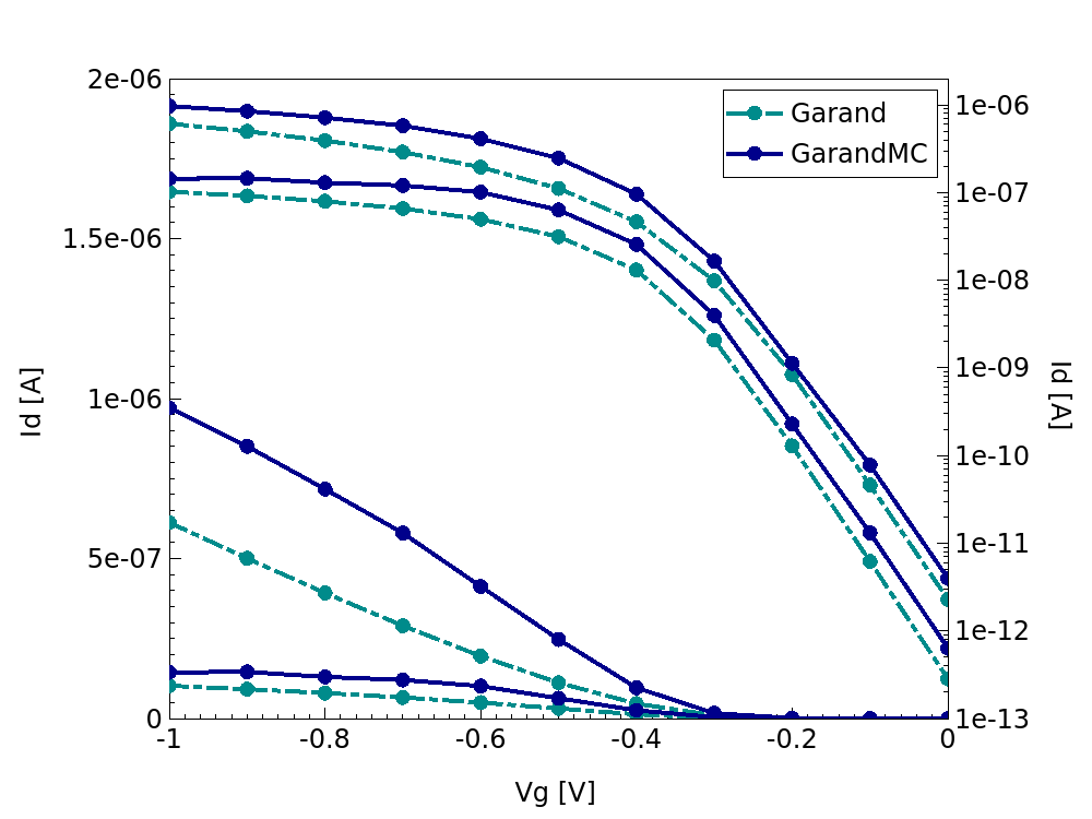
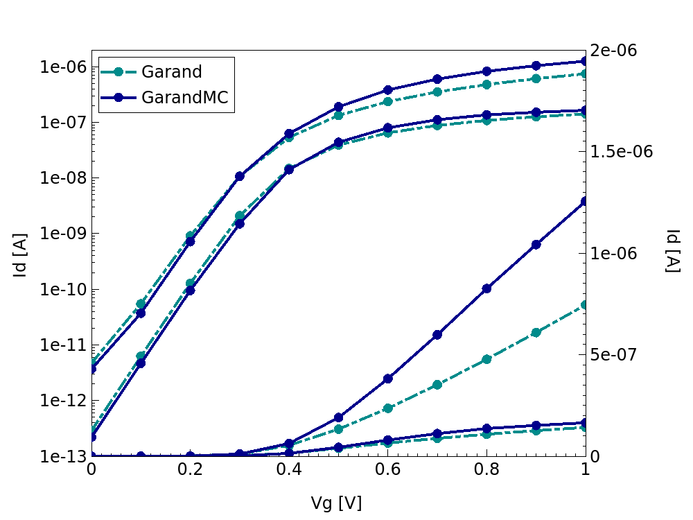
Figure 9. I_D-V_G characteristics for the PMOS (left) and NMOS (right) device simulation from both the initial drift-diffusion simulation and the Garand MC transport simulation.

Figure 10 shows the electron density from drift-diffusion and Monte Carlo simulation of the NMOS device at V_D=V_G=1.0V. This is averaged over time and the semiconductor cross section for each of the slices defined by the num_slices variable. Additionally, the electron velocity from the Monte Carlo simulation along the channel is shown, which is weighted by the carrier density. These are extracted using the results_MC stage.

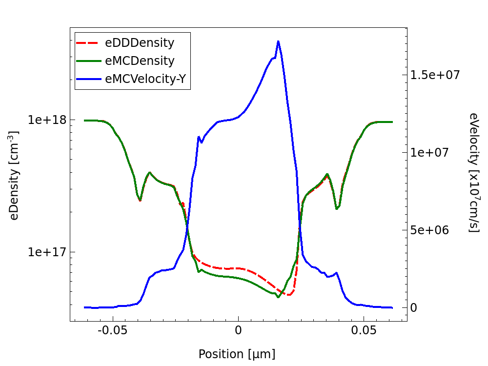
Figure 10. Electron density and velocity profile from Garand MC simulation of the nMOSFET at V_D=V_G=1.0V.